Data scientists who come to the career without a software background tend to use a procedural style of programming rather than taking an object oriented approach. Changing styles is a paradigm shift and really takes some time to wrap your mind around. Many of us who have been doing this for years still have trouble envisioning how objects can improve things.
The objective of this notebook is to apply Object Oriented Programming (OOP) via Machine Learning approach (by using Linear Regression models as an example here) for Data Science problems.
# Base libraries
import os
import time
import datetime
import json
import logging

# Scientific libraries
import numpy as np
import pandas as pd
from sklearn import svm # or any other function
from sklearn.datasets import load_boston
from sklearn.metrics import mean_squared_error
from sklearn.linear_model import LinearRegression as LR
from sklearn.linear_model import SGDRegressor as SGDR
from sklearn.preprocessing import StandardScaler
from sklearn.utils.validation import check_X_y, check_array

# Visual libraries
import matplotlib.pyplot as plt
from matplotlib import rcParams
import seaborn as sns
# most definitely plotly

# Helper libraries
from tqdm.notebook import tqdm, trange
from colorama import Fore, Back, Style
import warnings
warnings.filterwarnings('ignore')

# Visual setup
# plt.style.use('fivethirtyeight')   # alternatives below
plt.style.use("ggplot")
sns.set_style('darkgrid')
rcParams['axes.spines.right'] = False
rcParams['axes.spines.top'] = False
# plt.rcParams['figure.figsize'] = [10,6]
# rcParams["figure.autolayout"] = True
plt.rc('xtick', labelsize=11)
plt.rc('ytick', labelsize=11)
custom_colors = ['#74a09e','#86c1b2','#98e2c6','#f3c969','#f2a553', '#d96548', '#c14953']
sns.set_palette(custom_colors)
# custom_palette = ["#221f1f", "#b20710", "#e50914", "#f5f5f1"]
# sns.set_palette(custom_palette)
%config InlineBackend.figure_format = 'retina'

# Pandas options
# pd.set_option("max_colwidth", 100)
pd.set_option('max_colwidth', 40)
pd.set_option("display.precision", 4)
# pd.set_option("float_format", "{:.5f}".format)
# pd.options.display.max_columns = 12
# pd.options.display.max_columns = None  # Possible to limit
# pd.options.display.max_columns = None  # Possible to limit

from IPython.core.interactiveshell import InteractiveShell
InteractiveShell.ast_node_interactivity = 'all'

import logging
logging.basicConfig(
    format="%(asctime)s - %(message)s", datefmt="%d-%b-%y %H:%M:%S", level=logging.INFO
)

# Seed value for numpy.random
np.random.seed(14)
# Load the Boston Housing dataset
boston = load_boston()
X = boston.data
y = boston.target


# Load the Boston Housing dataset
boston = load_boston()
X = boston.data
y = boston.target

# Check for and handle missing values (NaN)
X = np.nan_to_num(X)

# Standardize the features to have mean=0 and std=1
scaler = StandardScaler()
X = scaler.fit_transform(X)
from abc import ABC, abstractmethod
import inspect

class BasePredictor (ABC):

    @abstractmethod
    def fit(self, X, y):
        """ Fit predictor.
        Parameters
        ----------
        X: (ndarray, sparse matrix) of shape (n_samples,, n_features)

        y: ndarray of shape (n_samples,)
           The input target values.

        Returns
        -------
        self : object
               Fitted estimator.
        """
        pass

    @abstractmethod
    def predict(self, X):
        """
        Parameters
        ----------
        X: (array-like, sparse matrix) of shape (n_samples, n_features)

        Returns
        -------
        y_pred : ndarray of shape (n_samples,)

        """
        pass

    # copied from sklearn
    @classmethod
    def _get_param_names(cls):
        """Get parameter names for the estimator"""
        # fetch the constructor or the original constructor before
        # deprecation wrapping if any
        init = getattr(cls.__init__, "deprecated_original", cls.__init__)
        if init is object.__init__:
            # No explicit constructor to introspect
            return []

        # introspect the constructor arguments to find the model parameters
        # to represent
        init_signature = inspect.signature(init)
        # Consider the constructor parameters excluding 'self'
        parameters = [
            p
            for p in init_signature.parameters.values()
            if p.name != "self" and p.kind != p.VAR_KEYWORD
        ]
        for p in parameters:
            if p.kind == p.VAR_POSITIONAL:
                raise RuntimeError(
                    "scikit-learn estimators should always "
                    "specify their parameters in the signature"
                    " of their __init__ (no varargs)."
                    " %s with constructor %s doesn't "
                    " follow this convention." % (cls, init_signature)
                )
        # Extract and sort argument names excluding 'self'
        return sorted([p.name for p in parameters])

    # copied from sklearn
    def get_params(self, deep=True):
        """
        Get parameters for this estimator.
        Parameters
        ----------
        deep : bool, default=True
            If True, will return the parameters for this estimator and
            contained subobjects that are estimators.
        Returns
        -------
        params : dict
            Parameter names mapped to their values.
        """
        out = dict()
        for key in self._get_param_names():
            value = getattr(self, key)
            if deep and hasattr(value, "get_params"):
                deep_items = value.get_params().items()
                out.update((key + "__" + k, val) for k, val in deep_items)
            out[key] = value
        return out

    def reset(self):
        """ A method for reseting the predictor """
        new = self.__class__(**self.get_params())

    def load_params(self, params):
        """ A method to load model configuration.

        Parameters
        ----------
        param : dict of parameters

        Returns
        -------
        A new model instance with the new parameters.

        """
        self = self.__class__(**params)
        print("params loaded")

        return self
class Data_plots():

    def __init__():
        pass

    def pairplot(self):
        '''Creates pairplot of all variables and the target using the Seaborn library'''

        print ("This may take a little time. Have patience...")
        from seaborn import pairplot
        from pandas import DataFrame
        df = DataFrame(np.hstack((X,y.reshape(-1,1))))
        pairplot(df)
        plt.show()

    def plot_fitted(self,reference_line=False):
        """
        Plots fitted values against the true output values from the data

        Arguments:
        reference_line: A Boolean switch to draw a 45-degree reference line on the plot
        """
        plt.title("True vs. fitted values",fontsize=14)
        plt.scatter(y,self.fitted,s=100,alpha=0.75,color='red',edgecolor='k')
        if reference_line:
            plt.plot(y,y,c='k',linestyle='dotted')
        plt.xlabel("True values")
        plt.ylabel("Fitted values")
        plt.grid(True)
        plt.show()
class Metrics():

    def mean_squared_err(self, y, y_pred):
        error = np.subtract(y, y_pred)
        squared_error = error ** 2
        return np.mean(squared_error)

    def root_mean_squared_err(self, y, y_pred):
        return np.sqrt(mean_squared_err)

    def mean_absolute_err(self, y, y_pred):
        error = np.subtract(y, y_pred)
        abs_error = np.abs(error)
        return np.mean(abs_error)
In linear regression we want to model the relationship between a scalar dependent variable $y$ and one or more independent (predictor) variables $\boldsymbol{x}$.
Given:
Assumptions:
Model:
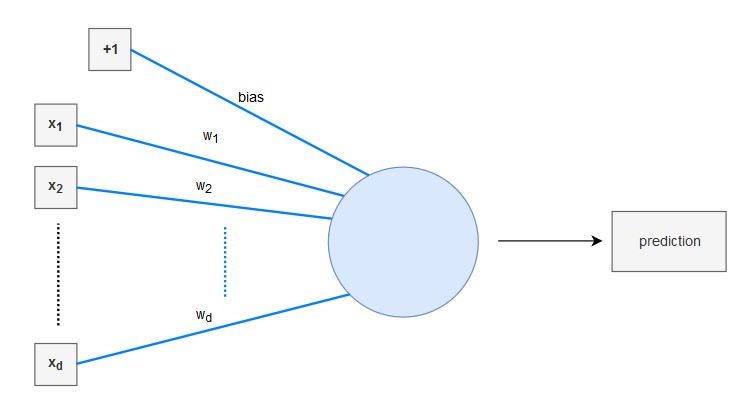
The linear regression model can be interpreted as a very simple neural network:
Approach:
Our goal is to learn the underlying function $f$ such that we can predict function values at new input locations. In linear regression, we model $f$ using a linear combination of the input features:
Our goal is to learn a linear model $\hat{y}$ that models $y$ given $X$.
$\hat{y} = XW + b$
The normal equation (closed-form solution): $\boldsymbol{w} = (\boldsymbol{X}^T \boldsymbol{X})^{-1} \boldsymbol{X}^T \boldsymbol{y}$
import numpy as np
from sklearn.utils.validation import check_X_y, check_array

class LinearRegression(BasePredictor, Data_plots, Metrics): # Class Inheritance
    def __init__(self, set_intercept = True):
        self.set_intercept = set_intercept
        self.intercept = None
        self.coefficients = None

    def fit(self, X, y):
        X, y = check_X_y(X, y) # checking if both X & y has correct shape
                               # and converting X, y into 2-d amd 1-d array
                               # even pandas dataframe get coverted into arrays
        if self.set_intercept == True:
            X_ = np.c_[np.ones((X.shape[0], 1)), X] # adding x0 = 1
        else:
            X_ = X
        self.beta = np.linalg.inv(X_.T.dot(X_)).dot(X_.T).dot(y)
        if self.set_intercept == True:
            self.coefficients = self.beta[1:]
            self.intercept = self.beta[0]
        else:
            self.coefficients = self.beta
        return self
    def predict(self, X):
        X_ = check_array(X) # validate the input, convert into 2-d numpy array
        self.fitted = X_@self.coefficients + self.intercept
        return self.fitted
Compare the predictions $\hat{y}$ with the actual target values $y$ using the objective (cost) function to determine the loss $J$. A common objective function for linear regression is mean squarred error (MSE). This function calculates the difference between the predicted and target values and squares it.
lr = LinearRegression()
lr.fit(X, y)
pred = lr.predict(X)
lr.mean_squared_err(y, pred)
<__main__.LinearRegression at 0x1f7bcc10a90>
21.894831181729202
Compare with Sklearn LinearRegression model
lr_2 = LR()
lr_2.fit(X, y)
pred2 = lr_2.predict(X)
mean_squared_error(pred2, y)
LinearRegression()
21.894831181729206
lr.plot_fitted(reference_line=True)

lr.get_params()
lr.intercept
lr.coefficients
{'set_intercept': True}
22.532806324110677
array([-0.92814606,  1.08156863,  0.1409    ,  0.68173972, -2.05671827,
        2.67423017,  0.01946607, -3.10404426,  2.66221764, -2.07678168,
       -2.06060666,  0.84926842, -3.74362713])
Calculate the gradient of loss $J(\theta)$ w.r.t to the model weights.
Update the weights $W$ using a small learning rate $\alpha$.
class LinearRegressionGD(BasePredictor, Data_plots, Metrics): # Class Inheritance
    def __init__(self, learning_rate=0.01, n_iterations=1000):
        self.learning_rate = learning_rate
        self.n_iterations = n_iterations
        self.coefficients = None
        self.intercept = None
        self.cost_history = []

    def fit(self, X, y):
        X, y = check_X_y(X, y)
        n_samples, n_features = X.shape
        self.coefficients = np.zeros(n_features)
        self.intercept = 0

        for i in range(self.n_iterations):
            # Predictions
            y_pred = np.dot(X, self.coefficients) + self.intercept

            # Calculate the gradient with respect to weights and bias
            dw = (1 / n_samples) * np.dot(X.T, (y_pred - y))
            db = (1 / n_samples) * np.sum(y_pred - y)

            # Update weights and bias
            self.coefficients -= self.learning_rate * dw
            self.intercept -= self.learning_rate * db

            # Calculate the cost (Mean Squared Error)
            cost = (1 / (2 * n_samples)) * np.sum((y_pred - y) ** 2)
            # if i  % 100 == 0:
            #     self.cost_history.append(cost)
            self.cost_history.append(cost)

    def predict(self, X):
        X = check_array(X)
        self.fitted = np.dot(X, self.coefficients) + self.intercept
        return self.fitted
lrgd = LinearRegressionGD(learning_rate=0.1, n_iterations=10000)
lrgd.fit(X, y)
pred = lrgd.predict(X)
lrgd.mean_squared_err(y, pred)
21.894831181729202
Compare with Sklearn SGDRegressor model
lrgd_2 = SGDR()
lrgd_2.fit(X, y)
pred_2 = lrgd.predict(X)
mean_squared_error(pred_2, y)
SGDRegressor()
21.894831181729202
lrgd.get_params()
lrgd.intercept
lrgd.coefficients
{'learning_rate': 0.1, 'n_iterations': 10000}
22.532806324110666
array([-0.92814606,  1.08156863,  0.1409    ,  0.68173972, -2.05671827,
        2.67423017,  0.01946607, -3.10404426,  2.66221764, -2.07678168,
       -2.06060666,  0.84926842, -3.74362713])
lrgd.plot_fitted(reference_line=True)