Play games first …

# set a seed for reproducible results
set.seed(1234)
# toss a coin
sample(c("H", "T"), 10, replace = TRUE)

##  [1] "H" "T" "T" "T" "T" "T" "H" "H" "T" "T"

# roll a die
sample(1:6, 10, replace = TRUE)

##  [1] 5 4 2 6 2 6 2 2 2 2

# roll 2 dice
dice = as.vector(outer(1:6, 1:6, paste))
sample(dice, 5, replace = TRUE)

## [1] "6 2" "5 2" "6 1" "2 1" "2 2"

# pick 6 of 54 - lottery
sample(1:54, 6)

## [1] 44 28 48 43  3 23

# play a card - a pair of jacks
cards = paste(rep(c("A", 2:10, "J", "Q", "K"), 4), c("H", "D", "S", 
    "C"))
sample(cards, 5)

## [1] "A D" "3 C" "K D" "9 H" "J H"

Back to normal stuffs …

# significant levels
alphas <- c(0.01, 0.05, 0.1, 0.32, 0.62)
# new function to plot significant levels with std. normal dist.
siglplot(alphas)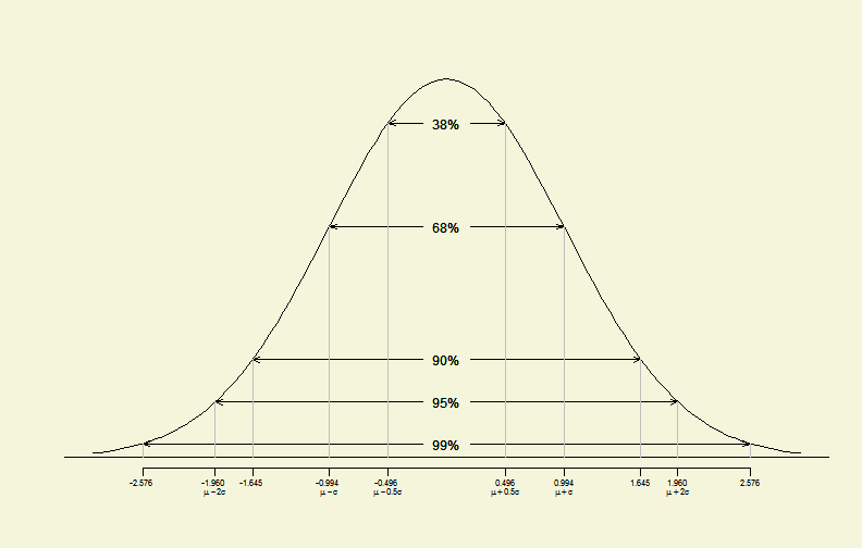

Standard Normal Distribution

Feel more confident …

# 2-sample - paired & !var.equal
x1 <- c(36.7, 35.8, 31.9, 29.3, 28.4, 25.7, 24.2, 22.6, 21.9, 20.3)
x2 <- c(36.2, 35.7, 32.3, 29.6, 28.1, 25.8, 23.9, 22, 21.5, 20)
# new function created by my own confidence :)
out <- ci.t(x1, x2, paired = TRUE, conf.level = c(0.9, 0.95, 0.99))
# using xtable to automatically generate a table as below:

# 95% confidence intervals includes population mean assume that population
# variance is known and its distribution is normal
smpsize <- 1000
obs <- 5

pmean <- 100
psd <- 5
conf.level <- 0.95

set.seed(1234)
d <- matrix(NA, obs, smpsize)
d <- replicate(smpsize, rnorm(obs, pmean, psd))
smean <- colMeans(d)
z.value <- qnorm(1 - (1 - conf.level)/2)
cil <- smean - z.value * psd/sqrt(obs)
ciu <- smean + z.value * psd/sqrt(obs)
sum(cil < pmean & ciu > pmean)/smpsize

## [1] 0.951

Test hypos …

A picture is worth a thousand words!

# 1-sample - 1-side
set.seed(1234)
x <- rnorm(130, mean = 2, sd = 3)
tres <- t.test(x, mu = 1, conf.level = 0.9, alternative = "greater")
# new plot function created to plot hypo. tests
plot(tres)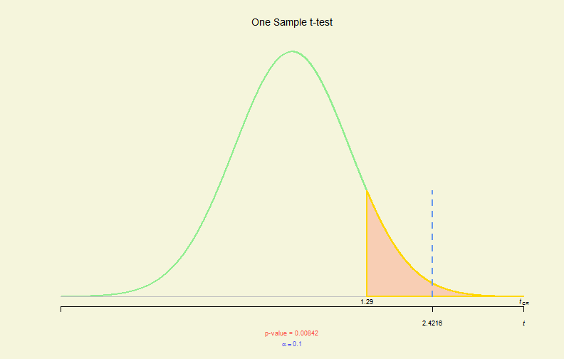

Hypo. Test Plot (I)

# 2-sample - 2- side, !paired & var.equal
myData <- read.csv("BeerWater.csv")
tres <- with(myData, t.test(B, W, var.equal = FALSE))
plot(tres)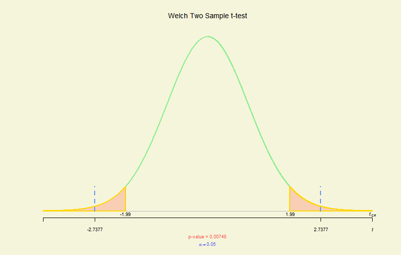

Hypo. Test Plot (II)

# 2-sample - 2-side, paired & !var.equal
x1 <- c(36.7, 35.8, 31.9, 29.3, 28.4, 25.7, 24.2, 22.6, 21.9, 20.3)
x2 <- c(36.2, 35.7, 32.3, 29.6, 28.1, 25.8, 23.9, 22, 21.5, 20)
tres <- t.test(x1, x2, paired = TRUE)
plot(tres)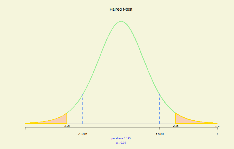

Hypo. Test Plot (III)

# 2-sample - 1-side, paired & !var.equal
x1 <- c(89, 87, 70, 83, 67, 71, 92, 81, 97, 78, 94, 79)
x2 <- c(94, 91, 68, 88, 75, 66, 94, 88, 96, 88, 95, 87)
tres <- t.test(x1, x2, alternative = "less", paired = TRUE)
plot(tres)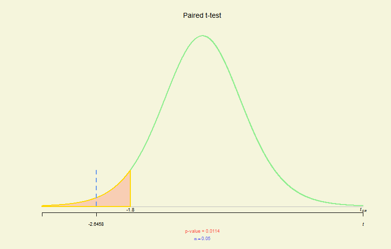

Hypo. Test Plot (IV)

# prop.test
pres <- prop.test(x = 18, n = 30, p = 0.55, alternative = "two.sided", 
    conf.level = 0.95, correct = FALSE)
plot(pres)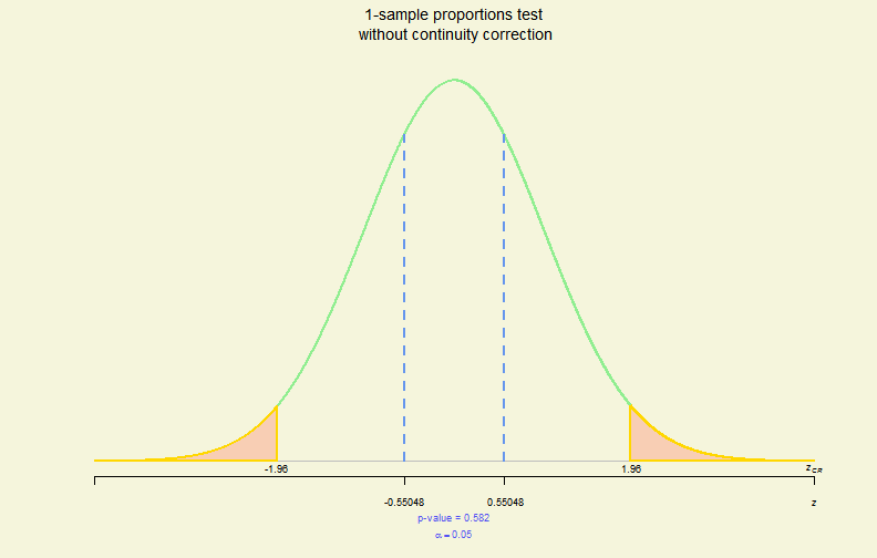

Hypo. Test Plot (V)

# var.test
myData <- read.csv("TeachingMethods.csv")
vres <- with(myData, var.test(E, L, alternative = "greater"))
plot(vres)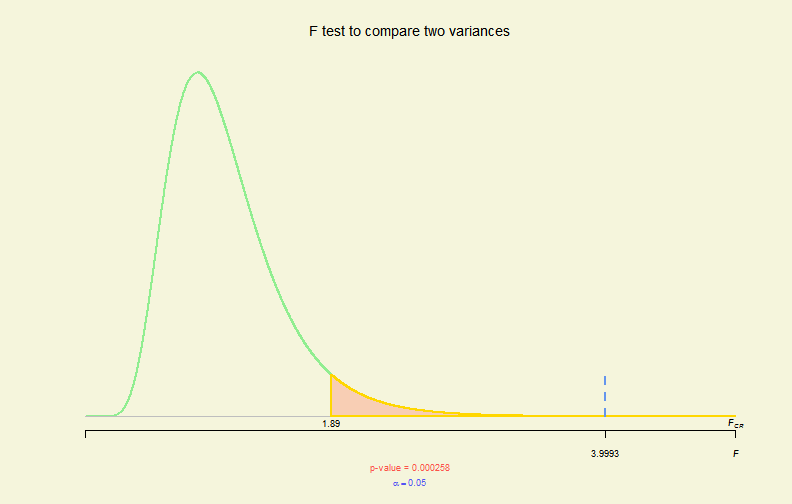

Hypo. Test Plot (VI)

Against power …

# 1-sample test on a population mean
power.t.test(n = 10, d = (70 - 60), sd = sqrt(400), sig.level = 0.05, 
    type = "one.sample", alternative = "two.sided")

## 
##      One-sample t test power calculation 
## 
##               n = 10
##           delta = 10
##              sd = 20
##       sig.level = 0.05
##           power = 0.2928
##     alternative = two.sided
## 

# 2-sample test on paired population mean differences
power.t.test(n = 5, d = 5, sd = 10 * sqrt(2 * (1 - 0.8)), sig.level = 0.05, 
    type = "paired", alternative = "one.sided")

## 
##      Paired t test power calculation 
## 
##               n = 5
##           delta = 5
##              sd = 6.325
##       sig.level = 0.05
##           power = 0.4296
##     alternative = one.sided
## 
##  NOTE: n is number of *pairs*, sd is std.dev. of *differences* within pairs 
## 

Categorical ones …

JG <- matrix(c(450, 20, 40, 40, 330, 40, 20, 40, 20), byrow = TRUE, 
    nrow = 3)
dimnames(JG) <- list(J1 = c("T", "F", "N"), J2 = c("T", "F", "N"))
print(JG)

##    J2
## J1    T   F  N
##   T 450  20 40
##   F  40 330 40
##   N  20  40 20

library(gmodels)
CrossTable(JG, expected = TRUE, prop.r = FALSE, prop.c = FALSE, prop.t = FALSE, 
    prop.chisq = FALSE, format = "SPSS")

## 
##    Cell Contents
## |-------------------------|
## |                   Count |
## |         Expected Values |
## |-------------------------|
## 
## Total Observations in Table:  1000 
## 
##              | J2 
##           J1 |        T  |        F  |        N  | Row Total | 
## -------------|-----------|-----------|-----------|-----------|
##            T |      450  |       20  |       40  |      510  | 
##              |  260.100  |  198.900  |   51.000  |           | 
## -------------|-----------|-----------|-----------|-----------|
##            F |       40  |      330  |       40  |      410  | 
##              |  209.100  |  159.900  |   41.000  |           | 
## -------------|-----------|-----------|-----------|-----------|
##            N |       20  |       40  |       20  |       80  | 
##              |   40.800  |   31.200  |    8.000  |           | 
## -------------|-----------|-----------|-----------|-----------|
## Column Total |      510  |      390  |      100  |     1000  | 
## -------------|-----------|-----------|-----------|-----------|
## 
##  
## Statistics for All Table Factors
## 
## 
## Pearson's Chi-squared test 
## ------------------------------------------------------------
## Chi^2 =  650.7     d.f. =  4     p =  1.609e-139 
## 
## 
##  
##        Minimum expected frequency: 8 
## 

library(vcd)
agreementplot(t(JG))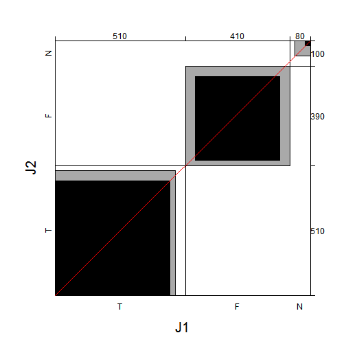

Plot of Agreement

summary(assocstats(as.table(JG)))

## 
## Number of cases in table: 1000 
## Number of factors: 2 
## Test for independence of all factors:
##  Chisq = 651, df = 4, p-value = 2e-139
##                     X^2 df P(> X^2)
## Likelihood Ratio 753.96  4        0
## Pearson          650.74  4        0
## 
## Phi-Coefficient   : 0.807 
## Contingency Coeff.: 0.628 
## Cramer's V        : 0.57 
## 

More classes in life …

data <- read.csv("Titanic.csv")
# who survived in the Titanic tragedy
library(ggplot2)
qplot(Class, data = data, geom = "bar", fill = Survived, postion = "stack", 
    facets = ~Sex) + coord_flip()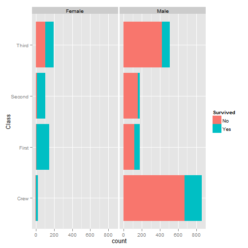

Plot of Facets

# survival rate
fun <- function(x) length(x[x == "Yes"])
t1 <- data.frame(with(data, aggregate(x = Survived, by = list(Class, 
    Sex, Age), FUN = length)))
t2 <- data.frame(with(data, aggregate(x = Survived, by = list(Class, 
    Sex, Age), FUN = fun)))
t1$y <- t2$x
t1$survived <- round(t1$y/t1$x, digits = 2)
t1[order(t1$survived, decreasing = T), ]

##    Group.1 Group.2 Group.3   x   y survived
## 9    First  Female   Child   1   1     1.00
## 10  Second  Female   Child  13  13     1.00
## 12   First    Male   Child   5   5     1.00
## 13  Second    Male   Child  11  11     1.00
## 2    First  Female   Adult 144 140     0.97
## 1     Crew  Female   Adult  23  20     0.87
## 3   Second  Female   Adult  93  80     0.86
## 4    Third  Female   Adult 165  76     0.46
## 11   Third  Female   Child  31  14     0.45
## 6    First    Male   Adult 175  57     0.33
## 14   Third    Male   Child  48  13     0.27
## 5     Crew    Male   Adult 862 192     0.22
## 8    Third    Male   Adult 462  75     0.16
## 7   Second    Male   Adult 168  14     0.08

And some factor(s) …

# one-factor ANOVA
x <- factor(c(rep("B", 5), rep("A", 5), rep("P", 5)), level = c("B", 
    "A", "P"))
y <- c(35, 25, 73, 45, 22, 36, 45, 22, 33, 14, 66, 97, 90, 76, 71)
library(ggplot2)
qplot(x, y, geom = "boxplot", fill = x)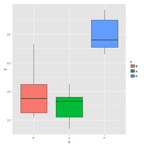

Boxplot (I)

summary(aov(y ~ x))

##             Df Sum Sq Mean Sq F value  Pr(>F)    
## x            2   7000    3500    14.2 0.00069 ***
## Residuals   12   2960     247                    
## ---
## Signif. codes:  0 '***' 0.001 '**' 0.01 '*' 0.05 '.' 0.1 ' ' 1 

# two-factor ANOVA
T <- factor(rep(rep(1:2, c(5, 5)), 3))
levels(T) <- c("D", "N")
P <- factor(rep(1:3, c(10, 10, 10)))
levels(P) <- c("B", "A", "P")
y <- c(35, 25, 73, 45, 22, 31, 55, 36, 49, 44, 36, 45, 22, 33, 14, 
    65, 44, 75, 62, 54, 66, 97, 90, 76, 71, 90, 77, 55, 72, 76)
library(ggplot2)
qplot(P, y, geom = "boxplot", fill = T)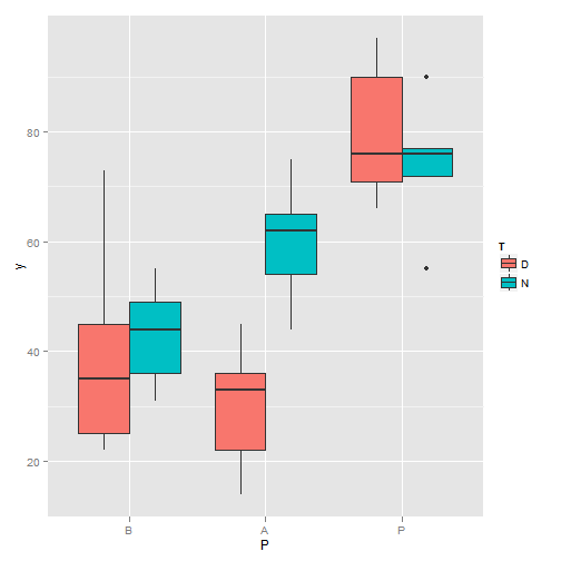

Boxplot (II)

qplot(T, y, geom = "boxplot", fill = P)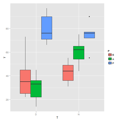

Boxplot(III)

summary(aov(y ~ T * P))

##             Df Sum Sq Mean Sq F value  Pr(>F)    
## T            1    608     608    3.23   0.085 .  
## P            2   7655    3828   20.35 6.8e-06 ***
## T:P          2   1755     877    4.67   0.019 *  
## Residuals   24   4514     188                    
## ---
## Signif. codes:  0 '***' 0.001 '**' 0.01 '*' 0.05 '.' 0.1 ' ' 1 

Simple (maybe) regression …

myData <- data.frame(x = c(31, 25, 29, 20, 40, 32, 27, 33, 28, 21), 
    y = c(58, 52, 61, 57, 93, 63, 68, 71, 73, 48))
# linear
m1 <- lm(y ~ x, data = myData)
library(ggplot2)
qplot(x, y, data = myData, geom = c("point", "smooth"), method = "lm")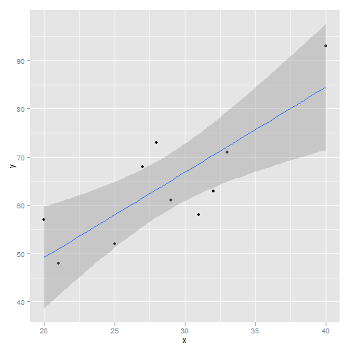

Plot of Linear Model

# log
m2 <- lm(y ~ log(x), data = myData)
# polynomial
m3 <- lm(y ~ poly(x, 2, raw = TRUE), data = myData)
# power
library(MASS)
bc <- boxcox(m1, plotit = FALSE)
lamda <- bc$x[which.max(bc$y)]
m4 <- lm(y ~ I(x^(1/lamda)), data = myData)
# exponential
f <- function(x, a, b) {
    a * exp(b * x)
}
fm <- nls(y ~ f(x, a, b), data = myData, start = c(a = 10, b = 0.1))
m5 <- lm(y ~ I(coef(fm)[1] * exp(coef(fm)[2] * x)) + 0, data = myData)

anova(m1, m2, m3, m4, m5)

## Analysis of Variance Table
## 
## Model 1: y ~ x
## Model 2: y ~ log(x)
## Model 3: y ~ poly(x, 2, raw = TRUE)
## Model 4: y ~ I(x^(1/lamda))
## Model 5: y ~ I(coef(fm)[1] * exp(coef(fm)[2] * x)) + 0
##   Res.Df RSS Df Sum of Sq    F Pr(>F)  
## 1      8 499                           
## 2      8 582  0       -83              
## 3      7 395  1       187 3.30  0.112  
## 4      8 768 -1      -372 6.59  0.037 *
## 5      9 443 -1       325              
## ---
## Signif. codes:  0 '***' 0.001 '**' 0.01 '*' 0.05 '.' 0.1 ' ' 1 

AIC(m1, m2, m3, m4, m5)

##    df   AIC
## m1  3 73.47
## m2  3 75.01
## m3  4 73.15
## m4  3 77.78
## m5  2 70.28

Multiple regression …

myData <- read.csv("exData.csv")
m1 <- lm(W ~ purchase + Q + N, data = myData)
library(ggplot2)
qplot(c(Q, N), W, data = myData, geom = c("point", "smooth"), col = purchase, 
    method = "lm", xlab = "Q+N")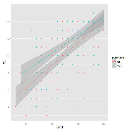

Plot of Linear Model

Travel with time …

load("STOCK.RData")
# plot prices with volumes
opar = par(mar = c(5, 4, 4, 5) + 0.1)
barplot(STOCK$Volume, col = "Gray", border = NA, axes = FALSE, axisnames = FALSE, 
    ylim = c(0, 5e+08))
axis(4)
mtext("Volume", side = 4, line = 3)
par(new = TRUE)
plot(STOCK$Adjusted, main = "STOCK", yaxt = "n")
axis(2)
mtext("Price", side = 2, line = 3)
par(opar)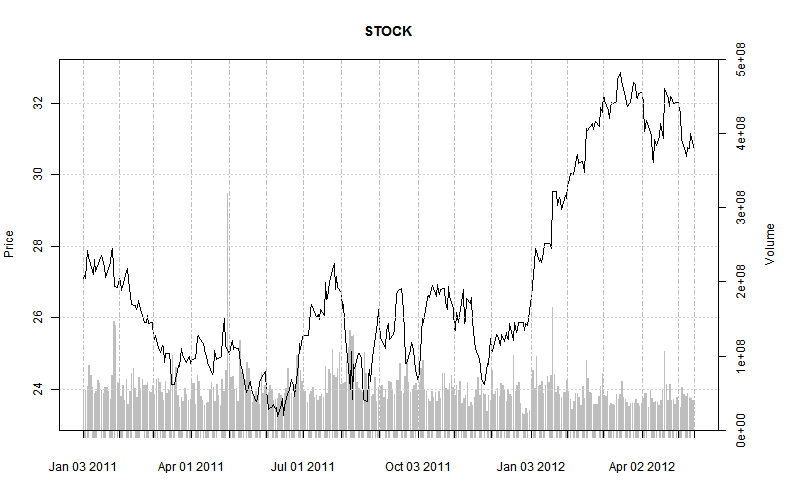

Plot of Time Series

Still have time …

# AR(3)
set.seed(1234)
n <- 200
x = arima.sim(model = list(ar = c(0.3, -0.7, 0.5), order = c(3, 0, 
    0)), n)
op <- par(mfrow = c(1, 2))
acf(x)
pacf(x)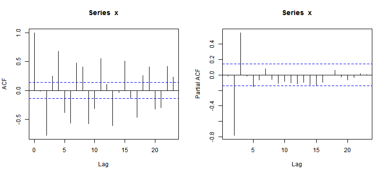

ACF and PACF Plot (I)

par(op)
Box.test(x, lag = log(n), type = "Ljung")

## 
##  Box-Ljung test
## 
## data:  x 
## X-squared = 261, df = 5.298, p-value < 2.2e-16
## 

y <- arima(x, order = c(3, 0, 0))
op <- par(mfrow = c(1, 2))
acf(y$resid)
pacf(y$resid)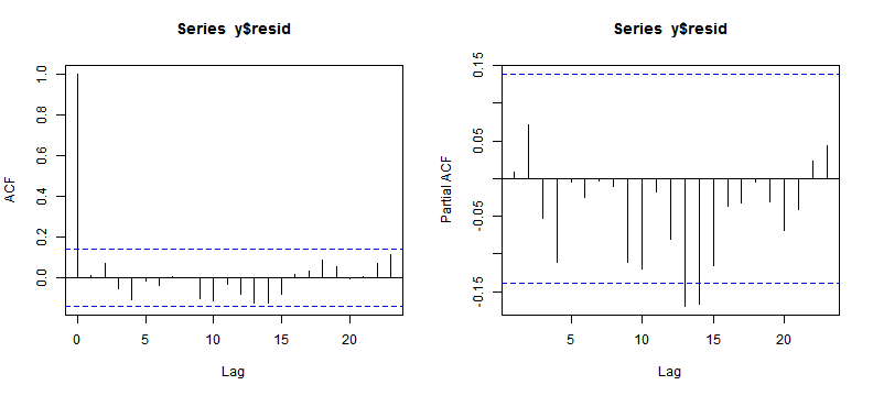

ACF and PACF Plot (II)

par(op)
confint(y)

##              2.5 %  97.5 %
## ar1        0.27746  0.5101
## ar2       -0.82847 -0.6851
## ar3        0.42134  0.6516
## intercept -0.01366  0.3107

library(forecast)
y <- auto.arima(x)
confint(y)

##               2.5 %  97.5 %
## ar1       -0.271553 -0.1638
## ar2       -0.989699 -0.8908
## ma1        0.467648  0.7678
## ma2        0.358998  0.6902
## ma3        0.097702  0.3812
## intercept  0.002771  0.2938

plot(forecast(y, h = 10, level = c(80, 95)))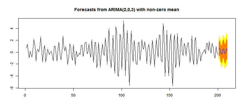

Time Series Plot with Forecasts

Bootstrap something final …

m1 <- lm(W ~ purchase + Q + N, data = myData)
set.seed(1234)
library(boot)
results <- boot(data = myData, statistic = bs, R = 1000, formula = W ~ 
    purchase + Q + N)
plot(results, index = 2)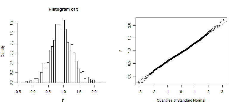

Density Plot and Q-Q Plot

confint(m1)

##                2.5 % 97.5 %
## (Intercept) -0.61275 2.4117
## purchaseYes  0.22564 1.6733
## Q            0.08631 0.3343
## N            0.42732 0.7539

boot.ci(results, type = "bca", index = 2)

## BOOTSTRAP CONFIDENCE INTERVAL CALCULATIONS
## Based on 1000 bootstrap replicates
## 
## CALL : 
## boot.ci(boot.out = results, type = "bca", index = 2)
## 
## Intervals : 
## Level       BCa          
## 95%   ( 0.2749,  1.7697 )  
## Calculations and Intervals on Original Scale

boot.ci(results, type = "bca", index = 3)

## BOOTSTRAP CONFIDENCE INTERVAL CALCULATIONS
## Based on 1000 bootstrap replicates
## 
## CALL : 
## boot.ci(boot.out = results, type = "bca", index = 3)
## 
## Intervals : 
## Level       BCa          
## 95%   ( 0.1050,  0.3179 )  
## Calculations and Intervals on Original Scale

boot.ci(results, type = "bca", index = 4)

## BOOTSTRAP CONFIDENCE INTERVAL CALCULATIONS
## Based on 1000 bootstrap replicates
## 
## CALL : 
## boot.ci(boot.out = results, type = "bca", index = 4)
## 
## Intervals : 
## Level       BCa          
## 95%   ( 0.4037,  0.7934 )  
## Calculations and Intervals on Original Scale

coef(m1)

## (Intercept) purchaseYes           Q           N 
##      0.8995      0.9495      0.2103      0.5906 

print(results)

## 
## ORDINARY NONPARAMETRIC BOOTSTRAP
## 
## 
## Call:
## boot(data = myData, statistic = bs, R = 1000, formula = W ~ purchase + 
##     Q + N)
## 
## 
## Bootstrap Statistics :
##     original    bias    std. error
## t1*   0.8995 -0.009424     0.77403
## t2*   0.9495 -0.013474     0.36631
## t3*   0.2103 -0.001269     0.05625
## t4*   0.5906  0.002895     0.09510

My sessionInfo …

print(sessionInfo(), locale = FALSE)

## R version 2.14.2 (2012-02-29)
## Platform: i386-pc-mingw32/i386 (32-bit)
## 
## attached base packages:
##  [1] tcltk     splines   parallel  grid      stats     graphics  grDevices
##  [8] utils     datasets  methods   base     
## 
## other attached packages:
##  [1] car_2.0-12            nnet_7.3-1            survival_2.36-12     
##  [4] quantmod_0.3-17       TTR_0.21-1            xts_0.8-6            
##  [7] Defaults_1.1-1        animation_2.0-6       boot_1.3-4           
## [10] forecast_3.21         RcppArmadillo_0.3.0.3 Rcpp_0.9.10          
## [13] fracdiff_1.4-1        tseries_0.10-28       zoo_1.7-7            
## [16] quadprog_1.5-4        ggplot2_0.9.0         vcd_1.2-13           
## [19] colorspace_1.1-1      MASS_7.3-17           gmodels_2.15.2       
## [22] xtable_1.7-0          knitr_0.5            
## 
## loaded via a namespace (and not attached):
##  [1] codetools_0.2-8    dichromat_1.2-4    digest_0.5.2      
##  [4] evaluate_0.4.2     formatR_0.4        gdata_2.8.2       
##  [7] gtools_2.6.2       highlight_0.3.1    lattice_0.20-6    
## [10] memoise_0.1        munsell_0.3        parser_0.0-14     
## [13] plyr_1.7.1         proto_0.3-9.2      RColorBrewer_1.0-5
## [16] reshape2_1.2.1     scales_0.2.0       stringr_0.6       
## [19] tools_2.14.2